Problem:
Have you tried copying a formula involving cells within a pivot table? You may find that the the value in the target cells don't change. You may also notice that the formula doesn't refrerence the cells in the usual way like A1, C2, etc. Instead, it uses the GetPivotData function. for example when I tried creating a formula adding J4 and I4 and that both J4 and I4 within a Pivot Table. But the formula you see in the target cell is something like the one below:
=GETPIVOTDATA("Sum of Dec'16"|$A$3|"Group"|"Administrative Expenses")+GETPIVOTDATA("Sum of Nov'16"|$A$3|"Group"|"Administrative Expenses")
As copying this formula to the adjoining cell does not change the cell reference and as such the value doesn't change. How do we workaround this issue?
Solution:
I am sure while creating the formula, you would have used the mouse to select the cells referenced in the formula. Try just typing the cell references in the formula without using the mouse. For instance, just type '=J4+I4' and there you go, the formula remains as it is and at this instance you don't see the reference to the GetPivotData function. Now you copy this formula to the adjoining cells and it works as usual and no issues. So the issue is when you select the cells referenced in the formula using the mouse / touch pad.
Now why Excel behaves like this, we don't know. However, if you don't like this behavior and permanently disable this you need to do this. It's simple.
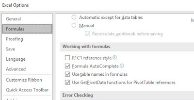
Bring up the Excel Options by clicking on File --> Options menu. May be, there are different ways of reaching out to the Excel Options in different versions of Excel. Under the Formulas Tab, you will find a check box 'Use GetPivotData functions for Pivot Table References' under Working with formulas section. Given below is a screen shot of Excel 2016.
There you go, just uncheck this checkbox and Excel won't use the GetPivotData function any more.
